


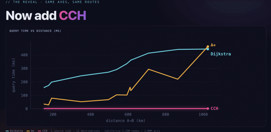
Most shortest path algorithms get slower as two points get farther apart. On a country-sized road map, a trip across town is cheap, but a cross-country route can cost hundreds of milliseconds.
FalkorDB supports three ways to find shortest paths: Dijkstra, A*, and Customizable Contraction Hierarchies (CCH). CCH is built in as an index. On a California road network with 1.25 million nodes and 3.06 million edges, it returns the longest route in the state in about 1 ms, and that number stays flat at any distance.
This post explains how each algorithm works, how they compare on the same map, and when to use each one.
The requirement: query time must not be significantly longer for longer routes
The work started with a request from a geospatial intelligence company. They were evaluating several graph databases to store country-sized road maps and run routing queries directly in the database.
They also had one hard requirement. As two points get farther apart, query time can grow at most linearly. If a 100 km route takes 100 ms, a 1,000 km route should take no more than 1,000 ms. A cross-country trip can’t cost 100 times a trip across town.
The first numbers didn’t clear that bar. Off-the-shelf shortest path scaled with the area searched, not the distance traveled, so long trips got expensive fast. The team spent the next stretch optimizing the algorithms FalkorDB already had, one at a time, measuring every change on a real map. Then they added a new one.
Not just a maps problem
This customer routes vehicles on roads, but the same cost curve shows up anywhere you traverse a large graph:
- Logistics: delivery and fleet routing, where every added stop multiplies the routing work.
- Networks and infrastructure: least-cost paths across telecom, power, and transit networks, or the fastest route for data across many hops.
- GenAI and RAG: connecting two entities in a knowledge graph is a shortest path query.
- Finance: following how money moves between accounts, and finding the short chains that reveal fraud rings.
In a road graph, nodes are intersections and edges are roads. Each edge carries a weight, such as distance, driving time, or a toll. A shortest path query finds the route with the lowest total weight.
Dijkstra: the baseline
Dijkstra’s algorithm is where most people start, and it was the first thing the team optimized. It works like this:
- Start at the source with a cost of 0.
- Always expand the unvisited node with the lowest known cost.
- Update the cost of each of its neighbors if this path is cheaper.
- Stop when the target becomes the lowest-cost node.
With positive edge weights, the lowest-cost node in the queue is final. Any other route to it would pass through a node that already costs more. That is why Dijkstra always returns the optimal path, with no precomputation and no extra knowledge of the graph.
The tradeoff is that it has no sense of direction. It only knows cost, so it expands outward in every direction like a growing circle around the source. The farther away the target is, the more of the map it has to explore before it gets there.
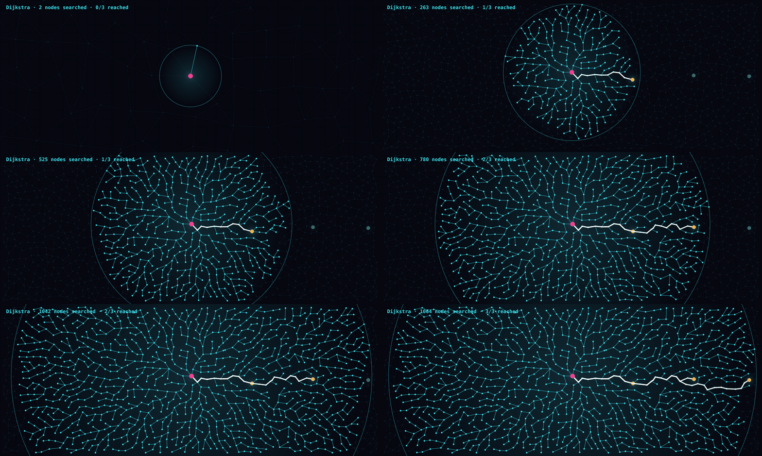
On the California network, with Los Angeles as the source, a 151 km route took 157 ms and a 1,025 km route took 443 ms. That clears the linear bar, but it is still hundreds of milliseconds per query, and every alternative route you ask for (K > 1) adds more.
A*: pointing the search at the goal
A* keeps Dijkstra’s guarantee and adds a hint about which way to go. Instead of expanding the node with the lowest cost so far, it expands the node with the lowest cost so far plus an estimate of the remaining distance:
f(n) = g(n) + h(n)
Here g(n) is the cost to reach node n and h(n) is the heuristic. On a road map, the natural heuristic is straight-line distance, as the crow flies. As long as the heuristic never overestimates the real remaining cost, A* still returns the optimal path. It just gets there while exploring far less of the graph, because the search is pulled toward the target.
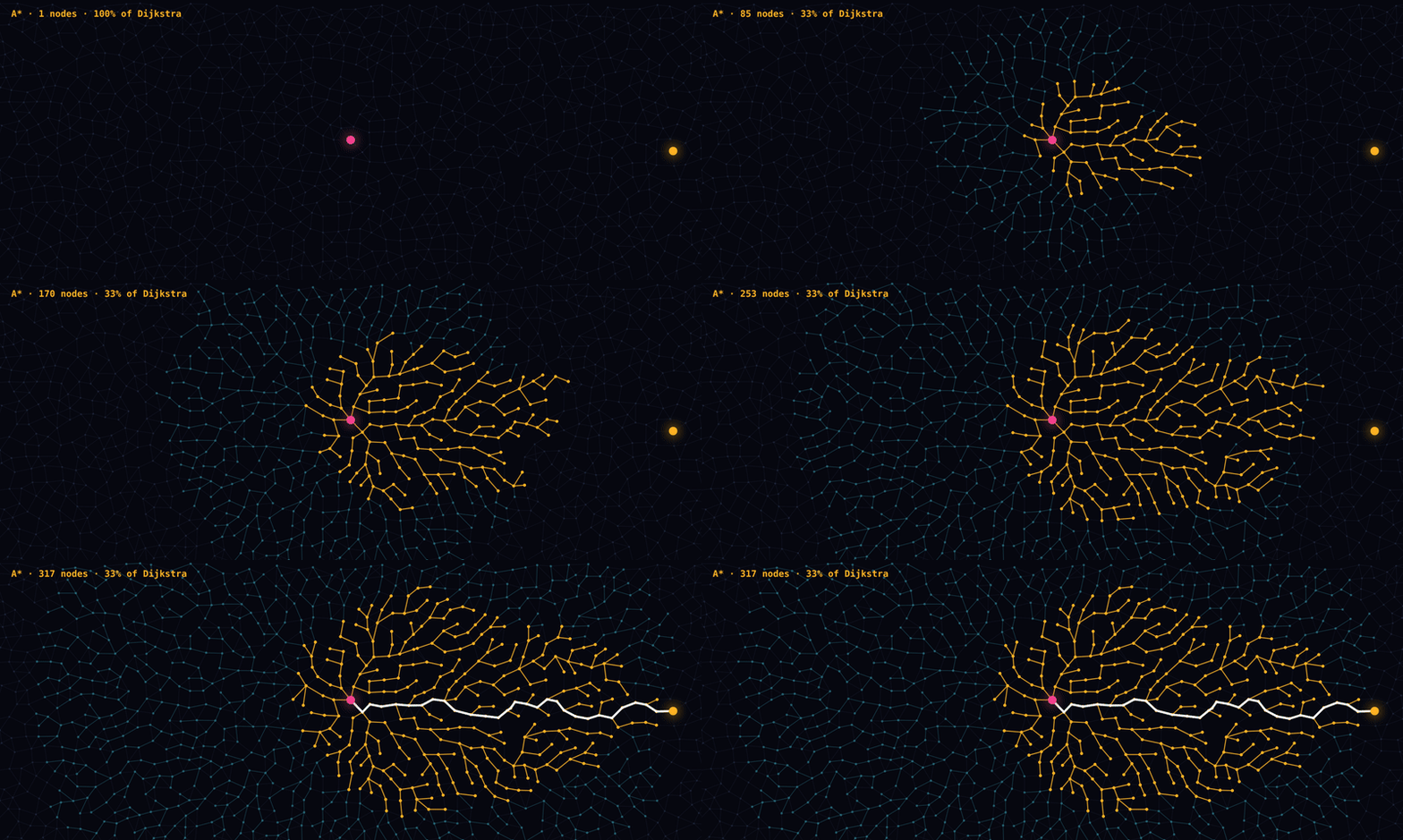
The heuristic is a simple value that can be computed between any two nodes as needed. On a road network, it is calculated directly from each intersection’s latitude and longitude. If you’re minimizing driving time instead of distance, a distance heuristic can be converted into a time heuristic so you keep the benefit.
On the same California routes, A* was 2 to 6 times faster than Dijkstra on most trips. Los Angeles to San Francisco took 160 ms with A* versus 356 ms with Dijkstra.
At the far edge of the map, the gain disappears. On the longest route, Los Angeles to Eureka, A* took 463 ms, about the same as Dijkstra. California is long and narrow, so on that trip the straight-line hint doesn’t rule out much of the map. A* is faster, but its query time still grows steeply with distance. Getting below that growth meant changing the approach.
CCH: move the work off the query
Tuning Dijkstra and A* kept both inside the linear bar, but every query still cost hundreds of milliseconds and grew with distance. To get a flat cost, the team had to stop doing all the work at query time. That is the idea behind Customizable Contraction Hierarchies, an established technique from routing research that FalkorDB now offers as a built-in index.
CCH does the hard work once, up front:
- Rank nodes by importance. Importance reflects how central a node is to the graph. On a road map, highway interchanges rank high and quiet side streets rank low.
- Contract nodes and add shortcuts. As lower-ranked nodes are contracted, CCH adds shortcut edges that summarize long stretches of road, each with a known cost.
A query then runs two searches at once, one forward from the source and one backward from the target. Each is essentially Dijkstra with one rule: it can only move to higher-ranked nodes, using shortcuts where they exist. The two searches climb toward the most important nodes until they meet. CCH picks the cheapest meeting point, then unpacks the shortcuts along that route back into the real edges.
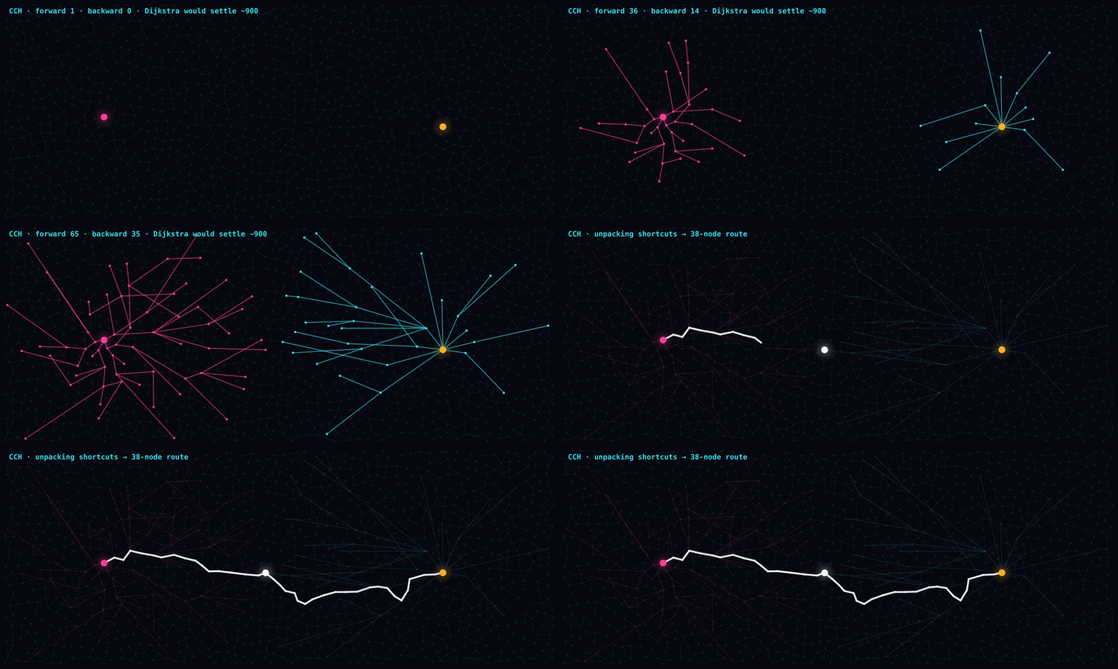
The result is that a query touches a tiny fraction of the graph, even when the graph is very large. On California, building the hierarchy takes about 5 seconds. Every query after that rides on it.
Why CCH is an index in FalkorDB
Databases already have a familiar way to trade a bit of upfront work for faster queries: the index. You build it once, the database keeps it in sync as data changes, and you never re-sync it by hand. FalkorDB already supports range, full-text, and vector indexes, so the team added CCH as one more index type.
The “customizable” part matters here. CCH separates the graph’s structure (which nodes connect to which) from its costs (distance, driving time, tolls). The structure is built once. The costs can be re-applied without a rebuild, which is what makes the index practical on data that changes.
In practice, a few kinds of change come up, and they cost very different amounts on the California network:
| Change | Example | Index update time |
|---|---|---|
| Update edge weights | Traffic on 1, 10, or 100 road segments | 0.3 ms, 0.9 ms, 16 ms |
| Close a road | Set its weight to a very high value | 0.9 ms |
| Remove an edge | Delete a road from the graph | 43 ms |
| Add an edge or node | A new road or intersection | About 5 s (full rebuild) |
Two practical notes came out of this. First, to model a road closure, raise its weight instead of deleting the edge. The road stays in the graph and the index absorbs the change in under a millisecond. Second, structural additions currently trigger a full rebuild. Those changes are rare on most road networks, and 5 seconds for a state-sized map is a reasonable cost.
Results: about 1 ms at any distance
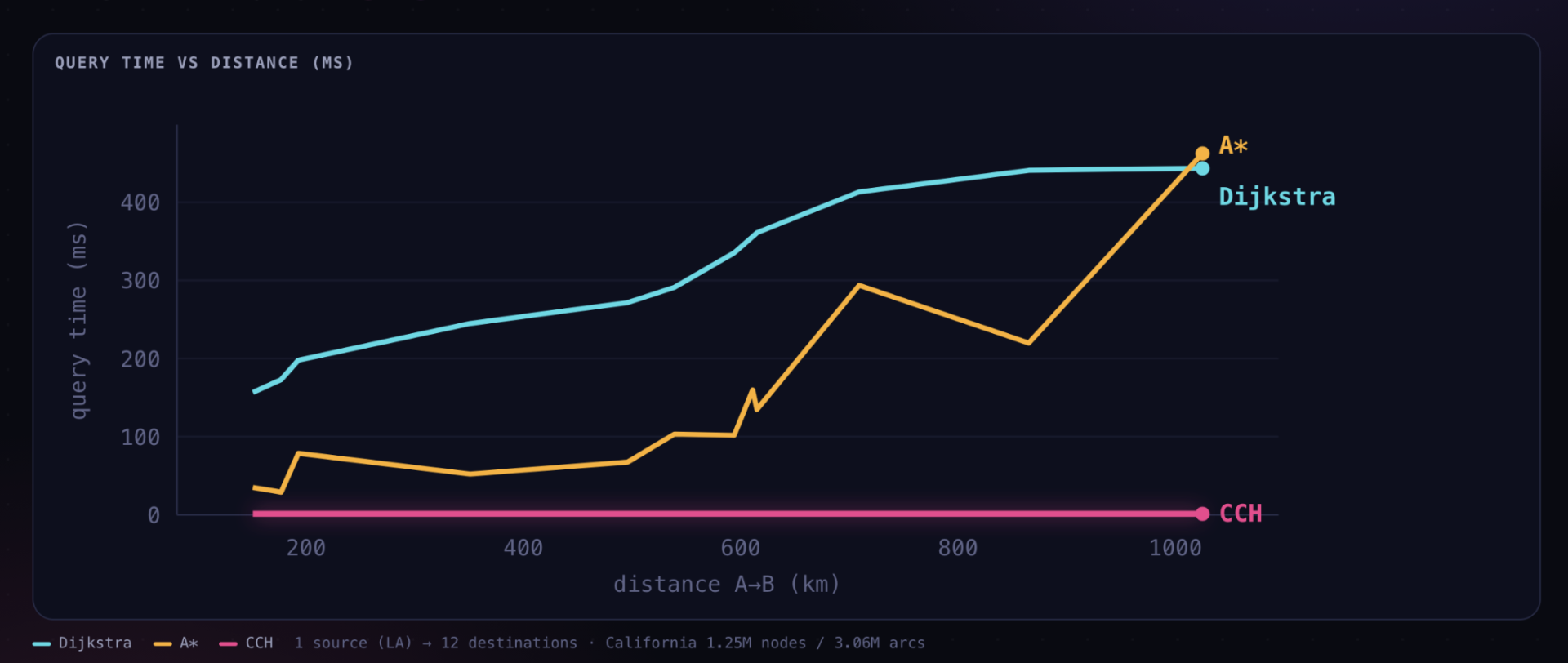
Before CCH, the fastest way to answer the longest California route was a full Dijkstra search at about 450 ms. Today the same route takes 1.08 ms through the CCH index, about 410 times faster, and alternative routes (K > 1) got much faster over the same period.
Memory follows the same pattern. Peak memory per query grew with distance for Dijkstra (59 MB to 235 MB) and A* (up to 135 MB), because both keep a queue of frontier nodes that widens as the search spreads. CCH used 0.05 MB per query on every route, and the index itself takes some memory to hold.
The same holds in an interactive routing demo on the California map. For a route from Redding to Los Angeles, CCH returned the shortest path in 11 ms, while A* took about 3 seconds to find two alternatives. Adding traffic to segments of that route updated the index in under 60 ms, and the rerouted query came back in under 6 ms with a new driving time.
The customer selected FalkorDB after an independent evaluation of several graph databases. Flat query time from CCH was a capability none of the other databases in the evaluation offered.
Which algorithm to use
CCH isn’t the right answer for every graph. Each one fits a different situation.
Use Dijkstra when you run shortest path occasionally or on a small graph. There is no index to build, it runs on any graph as-is, and it makes no assumptions about the data.
Use A* when your graph has information that can drive a good heuristic, such as coordinates on a map. It is a large improvement on geometric graphs, though its cost still grows with distance.
Use CCH when the graph is large, its structure is fairly stable, and you query it over and over with latency in mind. You pay a one-time build and some memory to hold the index, and in return queries stay around 1 ms at any distance.
Common questions
Why was FalkorDB a good fit for CCH?
FalkorDB stores graphs as sparse adjacency matrices in compressed sparse row (CSR) format. For Dijkstra and A*, that layout keeps related data close together in memory, which makes traversal faster and leaner. For CCH the benefit is larger. The centrality calculations used to rank nodes, and the graph dissection step, work directly on an adjacency matrix in CSR form. That is FalkorDB’s native format, so there was no conversion step.
How does FalkorDB handle super nodes?
In a sparse matrix, a super node is a row with many entries. Traversals run as sparse matrix operations on GraphBLAS, a parallel linear algebra engine, so a heavily connected node doesn’t degrade performance. With CCH, a central super node can even help. Think of a main cable connecting two continents: CCH ranks it high and builds shortcuts to it, so queries reach it quickly.
Can I restrict a shortest path to certain edge types?
Yes, when you create the CCH index. You specify which relationship types it should build on, for example roads but not trails, and anything outside that set is ignored at query time. Other filters during traversal aren’t supported yet.
Can I have more than one CCH index on the same graph?
Yes. You can create several CCH indexes on one graph and choose between them per query.
When do I build the index?
Whenever you want. You can start with Dijkstra or A*, see whether they are fast enough, and create a CCH index later if they aren’t. If it doesn’t help, you can drop it.
How do I know if CCH is a good option for me?
CCH is a good option if you have a stable network, whose nodes and edge structure don’t change often, with a hierarchical structure, where you need to perform many queries. In that case indexing with CCH can give great results. If you only perform one-off queries, or your network has an artificial structure such as a grid, Dijkstra or A* will likely be the better option.
What other graph algorithms does FalkorDB support, and can I add my own?
FalkorDB includes shortest path, community detection, and other algorithms such as weakly connected components, max flow, and DFS. The full list is in the docs. For anything not built in, FalkorDB supports user-defined functions in JavaScript, with APIs for reading nodes, edges, and neighbors, so you can write your own algorithm and load it into the database.
Try it on your own graph
FalkorDB is open source, and Dijkstra, A*, and CCH are all built in. The quickest way to start is the latest Docker image:
docker run -p 6379:6379 -p 3000:3000 -it --rm falkordb/falkordb:latestThe FalkorDB docs cover each algorithm, including how to create a CCH index. Two demos are on GitHub:
- CCH-demo: the California routing demo, with live traffic updates.
- game-pathfinding: real-time path recomputation on a grid as you add walls.
If you have questions about your own use case, reach out to the team.