

Some problems announce themselves as graph problems. Most don’t. A scheduler that can’t double-book reviewers, a fraud queue that keeps sending two analysts after the same cluster, a retrieval step that returns five near-identical passages. All three are the same question wearing different clothes: which items can I pick so that no two of them conflict?
The graph-theoretic answer is the independent set. The version that matters in production is the maximal independent set (MIS): a conflict-free selection that can’t be extended. It isn’t always the biggest such selection. It is fast, and in most operational systems that trade is worth making.
Table of Contents
When You Need Non-Conflicting Resources in a Network
A team lead schedules interviews and finds that several candidates can’t sit in adjacent slots because the same reviewers are involved. A wireless engineer assigns channels to towers and needs neighboring towers on different frequencies. A data engineer picks nodes for parallel processing and needs the selected vertices to stay disconnected so workers don’t collide on shared dependencies.
Three different domains, one graph pattern: select vertices with no edges between them.
Formally, an independent set is a set of vertices S where no edge of the graph has both endpoints in S. The set is maximal when every vertex outside S has at least one neighbor inside it, so nothing can be added without breaking independence. That is a local condition, and it is cheap to satisfy.
Two structural facts are worth carrying around, because they let you reuse tooling you may already have. The complement of an independent set is a vertex cover. And an independent set in a graph is a clique in that graph’s complement.
Why this keeps showing up in real systems
Any time a conflict can be drawn as an edge, MIS is in scope. Compiler and runtime schedulers use the same logic to avoid overlapping work. Distributed systems use it to spread load. Graph databases use it to carve a large problem into pieces that can be processed independently.
Security graphs are a good example: the same non-overlap idea keeps analysts from chasing the same connected cluster twice. If you’re already modeling access paths as relationships rather than rows, our guide to security graphs and cloud entitlements covers that modeling side in more depth.
Practical rule: if two candidates can’t be selected together, make that constraint an edge. Once the conflict graph is explicit, MIS stops being an abstraction and becomes a query.
Why practitioners care
The gap between “can’t add anything else” and “largest possible” is the gap between a fast operational choice and a genuinely hard optimization problem. Plenty of production workflows only need a stable, conflict-free subset: enough to kick off parallel jobs, cut duplicated effort, or spread coverage across a network. Naming the pattern is most of the work. After that, you stop reinventing a heuristic every time a selection problem shows up.
Maximal vs Maximum Independent Sets Explained
The two words are not interchangeable
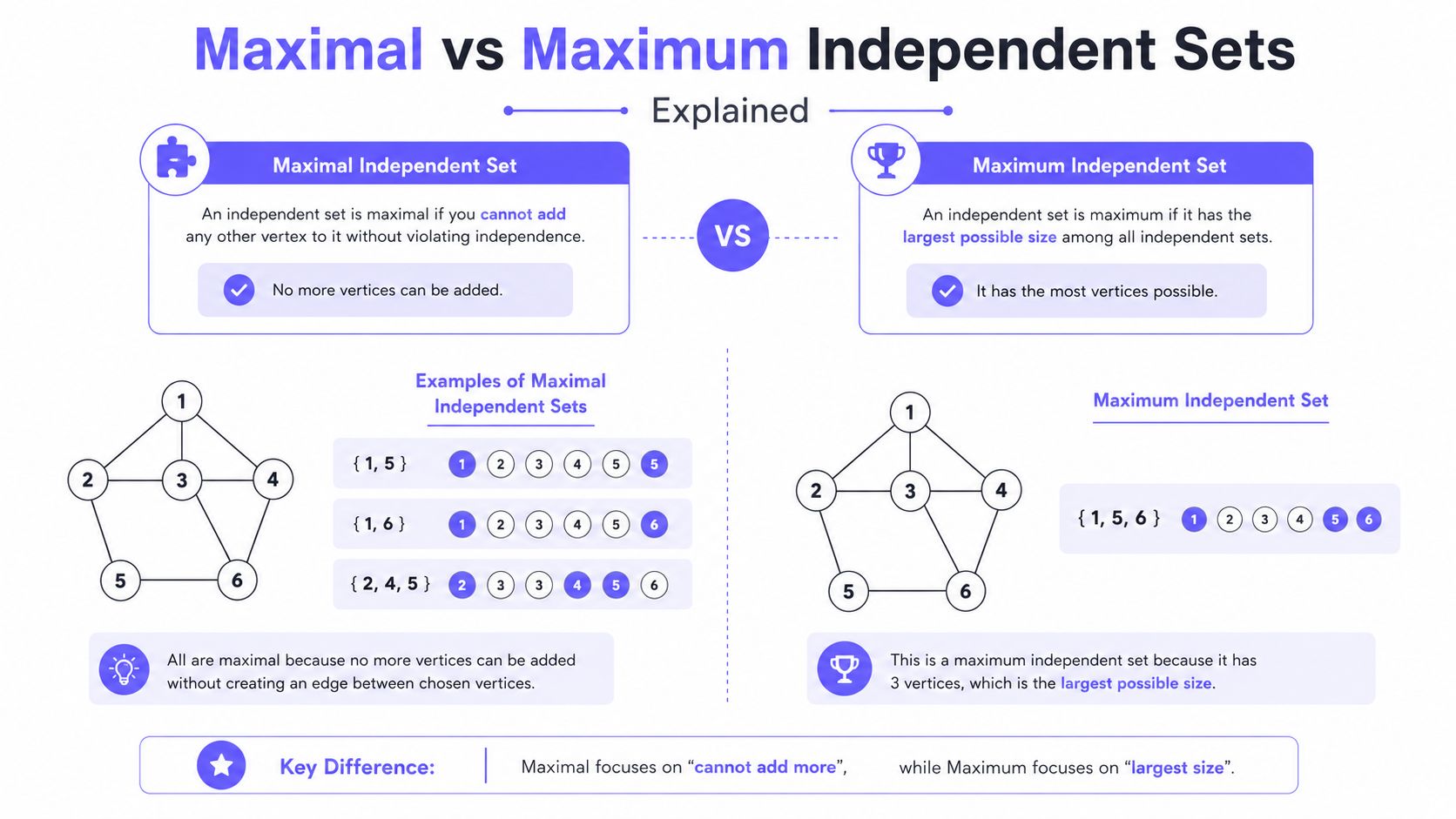
A maximal independent set cannot be extended. A maximum independent set is the largest independent set in the graph. The first is a local property, the second is a global optimum, and a graph can hold many maximal sets of very different sizes.
The smallest useful illustration is a five-vertex path, v1-v2-v3-v4-v5. The set {v1, v3, v5} is maximum, with three vertices. The set {v2, v4} is also maximal: v1, v3, and v5 each touch something already chosen, so none of them can be added. But it holds only two. Both are correct answers to “find a maximal independent set.” Only one answers “find the largest.”
The cost difference is not subtle. Computing a maximal independent set is linear in the size of the graph. Computing a maximum independent set is NP-hard, and it resists approximation: no polynomial-time algorithm gets within a factor of n^(1−ε) unless P = NP. That gap is the entire reason the vocabulary distinction earns its keep.
Which question are you really asking
-
Maximal: valid and non-extendable. Usually sufficient for operational workflows.
-
Maximum: largest by cardinality. Needed when the count itself is the value being delivered.
-
The common error: treating a greedy output as optimal because it happens to be legal.
A lot of production bugs trace back to exactly this mismatch. The algorithm did what it was designed to do; the requirement was written for a different problem.
Write the requirement down before writing the query. If the spec says “largest possible,” don’t ship “cannot be extended.” If the spec says “conflict-free coverage, quickly,” maximal is the right target and paying for a global search is waste.
Algorithm Families for Computing Maximal Independent Sets
Greedy is the default, and order matters
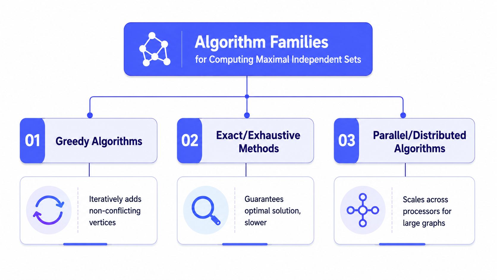
Walk the vertices, and add one only if it touches nothing already chosen. That’s the whole algorithm: O(n + m), easy to reason about, and usually the first thing anyone ships. It is also order-dependent, so the same graph yields different maximal sets under different traversal orders.
That dependence is a trade-off rather than a defect. Process high-degree vertices first and you can block a large share of the graph early, ending up with a small set. Randomize the order, or sort by ascending degree, and you avoid most pathological cases without turning the implementation into a research project.
Exact methods solve a different problem
Branch-and-bound search, ILP solvers, and Bron-Kerbosch over the complement graph all target the maximum independent set. They explore combinations systematically, prune invalid branches, and can prove optimality. The search cost grows fast enough to rule them out on large graphs. Their real home is small graphs, offline analysis, and generating ground truth to check a heuristic against.
Parameterized methods sit in between. When a graph has exploitable structure, such as bounded treewidth or planarity, specialized algorithms beat brute force by a wide margin. The catch is that they depend on those structural assumptions holding, which makes them excellent inside their niche and awkward outside it.
Parallel and distributed approaches are built for scale
MIS has been treated as a parallel problem since the 1980s, when Luby’s randomized algorithm showed it could be solved in O(log n) expected rounds, with each round selecting many vertices at once instead of one. Later work extended the idea to distributed and geometric settings, and to graphs too large for a single machine. The overview on maximal independent set algorithms is a reasonable starting point for that literature.
The round-based formulation matters for practical reasons beyond raw speed: it is set-oriented, which means it maps onto a query language far better than a per-vertex loop does. More on that in the next section.
| Approach | What it gives you | Best fit | What to watch |
|---|---|---|---|
| Sequential greedy | A valid maximal set in O(n + m) | Prototypes, small to mid-size graphs, application code | Output depends on vertex order |
| Exact search | The maximum independent set | Small graphs, offline optimization, verification | Search cost grows quickly |
| Round-based / parallel | Many vertices decided per round | Large graphs, database queries, distributed pipelines | Coordination and partition boundaries |
Implementing MIS in Graph Databases with Cypher
Cypher has no loop construct, and a vertex-at-a-time greedy pass is the wrong shape for a set-oriented query language anyway. The round-based formulation fits much better: each round is a single query that decides a whole batch of vertices, and a thin driver loop repeats it until nothing is left undecided.
The examples below use a fraud graph: :Account nodes joined by :CONFLICTS_WITH edges, where an edge means two accounts are too entangled to investigate separately.
Step 1: seed a random priority
MATCH (v:Account)
SET v.mis_state = 'undecided',
    v.mis_rank  = rand();
Step 2: select every local minimum
A vertex joins the set if no undecided neighbor outranks it. The comparison orders vertices by (mis_rank, ID) rather than rank alone, so two adjacent vertices that draw the same random value can never both qualify:
MATCH (v:Account {mis_state: 'undecided'})
OPTIONAL MATCH (v)-[:CONFLICTS_WITH]-(u:Account {mis_state: 'undecided'})
  WHERE u.mis_rank < v.mis_rank
     OR (u.mis_rank = v.mis_rank AND ID(u) < ID(v))
WITH v, count(u) AS betterNeighbors
WHERE betterNeighbors = 0
SET v.mis_state = 'selected'
RETURN count(v) AS newlySelected;
That second clause is what makes the query safe to copy into production. Because node IDs are unique, (mis_rank, ID) is a strict total order, which means every non-empty set of undecided vertices has exactly one minimum and no two neighbors can both see themselves as the local minimum. Drop the clause and a rand() collision between adjacent vertices selects both, producing an edge inside the result. That failure is rare enough to survive testing and awkward to debug afterward.
The same property guarantees termination: the globally lowest vertex always qualifies, so every round selects at least one node.
Step 3: block their neighbors
MATCH (:Account {mis_state: 'selected'})-[:CONFLICTS_WITH]-(u:Account {mis_state: 'undecided'})
SET u.mis_state = 'blocked'
RETURN count(DISTINCT u) AS newlyBlocked;
Step 4: drive the rounds
from falkordb import FalkorDB

g = FalkorDB(host="localhost", port=6379).select_graph("fraud")

g.query(SEED)

while g.query(SELECT_ROUND).result_set[0][0] > 0:
    g.query(BLOCK_ROUND)

selected = g.query(
    "MATCH (v:Account {mis_state:'selected'}) RETURN v.id ORDER BY v.id"
).result_set
With random ranks this converges in a logarithmic number of rounds on most real graphs, so even a large conflict graph tends to finish in single-digit or low double-digit iterations rather than millions.
One caveat on ID(). Internal identifiers are stable for the duration of a run, which is all the tie-break needs, but they can be reassigned after deletions and they carry no meaning outside the engine. If you want reproducible output, meaning the same input graph yields the same selected set every time, break ties on a domain key such as v.id and seed mis_rank from your application with a seeded generator instead of calling rand() in the query. Conversely, re-seeding with fresh randomness on each run yields a different valid maximal set, which is worth having when the first answer is legal but smaller than you’d like.
Verify the result
Two assertions confirm both halves of the definition. Independence:
MATCH (:Account {mis_state:'selected'})-[:CONFLICTS_WITH]-(:Account {mis_state:'selected'})
RETURN count(*) AS violations;  // expect 0
Maximality:
MATCH (v:Account) WHERE v.mis_state <> 'selected'
OPTIONAL MATCH (v)-[:CONFLICTS_WITH]-(s:Account {mis_state:'selected'})
WITH v, count(s) AS selectedNeighbors
WHERE selectedNeighbors = 0
RETURN count(v) AS notMaximal;  // expect 0
Both should return zero. Keep them in your test suite. They cost almost nothing and they catch the class of bug where a schema change quietly breaks the guarantee. They test the graph as recorded, though, not the world it describes, so there’s a third check worth adding on top of them. It’s covered under scaling below.
Variations worth knowing
| Approach | Cost profile | Best for | Pattern |
|---|---|---|---|
| Sequential greedy | One pass plus neighborhood checks | Small graphs, application-side control | Order vertices, check adjacency, mark selected |
| Degree-aware greedy | Greedy plus an ordering step | Dense or skewed graphs | Precompute degree, sort ascending, scan once |
| Randomized rounds | Logarithmic rounds, set-oriented | Large graphs inside the database | The pattern shown above |
| Local improvement | Extra passes over the result | Squeezing out a larger set | Swap a chosen vertex for two of its neighbors |
If you’re translating this into your own schema, our Cypher query cheatsheet covers the traversal and filtering syntax used above.
Keep the state small. MIS only needs to know three things per vertex: selected, blocked, or still undecided.
Real-World Applications in Production Systems
Nobody files a ticket asking for a maximal independent set. Fraud teams ask for non-overlapping investigation buckets. GraphRAG teams ask for context nodes that aren’t all from the same neighborhood. Security teams ask for coverage without redundant scans. MIS is the shape underneath all three requests.
Fraud detection and investigation triage
In fraud graphs, accounts, devices, cards, and IPs cluster tightly. Once an investigator picks one vertex out of a suspicious cluster, its neighbors make poor follow-up candidates, because they’re entangled in the same pattern and will surface much of the same evidence. A maximal independent set produces a shortlist that spreads analysts across distinct parts of the graph instead of stacking them on one dense pocket.
Queue triage is where this pays off. Rather than assigning every alert in a connected cluster to a different person, select a non-adjacent subset first and let the remainder wait for what the first pass reveals. The initial investigations usually change the graph anyway.
GraphRAG and context diversity
GraphRAG retrieval degrades when one tightly connected neighborhood dominates the results. With a fixed context budget, pulling five adjacent nodes often means paying five times for one fact.
MIS works well as a diversification filter here: it selects nodes far enough apart to widen coverage while keeping the set conflict-free. It doesn’t replace ranking or relevance scoring. It sits underneath them as a structural control, so the final context set isn’t overrun by a single cluster. The practical effect is more varied evidence and a better chance of covering different facets of the question.
Security analytics and asset sampling
Security graphs connect hosts, users, vulnerabilities, and alerts into dense relationships, and scanning capacity is always finite. A maximal independent set helps choose assets for scanning or validation without redundant overlap: if two nodes sit close together on the attack surface, checking both often means running nearly identical checks twice.
The idea travels beyond security. The GraphFrames 0.10.0 release added maximal independent set to its algorithm set, and cites a marketing use case: choosing non-overlapping influencers in a social network. Different vertical, identical structure: a coverage problem wearing a graph costume.
Performance Considerations and Scaling Strategies
Graph algorithms are cheap on a whiteboard and expensive in a live system. MIS exercises most of the usual pressure points at once, because every decision depends on neighborhood visibility. That makes storage layout at least as important as algorithm choice.
Architecture shapes the cost
The inner question never changes: is this vertex adjacent to something already selected? How expensive that question is depends entirely on how adjacency is stored.
FalkorDB represents the graph as sparse adjacency matrices and executes traversals as linear algebra over GraphBLAS, so a neighborhood check reads compact, contiguous structures instead of chasing pointers across scattered objects. For MIS, where that question is asked once per candidate per round, the difference compounds quickly. Our FalkorDB vs Neo4j performance benchmarks go into the measurement methodology.
Multi-tenancy deserves a mention too. When several teams share a platform, a simple greedy pass can turn noisy under concurrency without predictable interference control.
Structural independence is not semantic independence
MIS guarantees that no two selected vertices share an edge. It guarantees nothing about whether they represent different things in the real world. If a dirty ingest turns one person into three nodes, a structurally valid independent set can hand three copies of the same entity to three different analysts, and every check above still passes.
The mechanism is worse than simple bad luck, because fragmentation doesn’t merely permit duplicate selection. It encourages it. Splitting one entity across three nodes divides its edges among them, so each fragment carries a lower degree than the merged entity would. Low degree is exactly what every MIS heuristic rewards: degree-ascending greedy reaches fragments first, and in the randomized version a sparse node has fewer neighbors that can outrank it. The dirtier the ingest, the more the algorithm gravitates toward the artifacts of that dirt.
Missing edges compound it. The entire model rests on the premise that a conflict is an edge. When two records fail to resolve to the entities they belong to, the conflict between them was never written down, the algorithm sees two unrelated vertices, and it selects both. This is the failure mode the verification queries cannot catch, because they evaluate the graph as recorded rather than the world it stands for.
Over-merging is the mirror error and deserves equal weight. Resolution tuned too aggressively collapses two genuinely distinct entities into one node, which removes a legitimate candidate from the pool and folds two separate conflict sets into a single vertex. The result is a smaller set that looks cleaner and quietly covers less ground. Neither direction announces itself. Both surface downstream: two analysts opening the same case, GraphRAG returning three phrasings of one fact, a scanner probing the same host twice under different names.
The practical response is to resolve entities before building the conflict graph, and then to assert the result semantically as well as structurally. If nodes carry a resolved key, one more query closes the gap:
MATCH (v:Account {mis_state: 'selected'})
WITH v.entity_key AS entity, count(*) AS copies
WHERE copies > 1
RETURN entity, copies ORDER BY copies DESC;  // expect no rows
Run it alongside the independence and maximality checks. Together they cover both halves of the guarantee: the graph says these vertices don’t conflict, and the resolved keys say they aren’t the same thing twice.
All of which puts entity resolution inside this algorithm’s correctness surface rather than upstream of it. That applies to how records enter the graph, where collection pipelines and social data extraction APIs are a common source, and to the identity fields you resolve on, where something as ordinary as an email validation API keeps one contact from becoming three vertices with three spellings.
Scaling patterns that hold up
Parallelism is the next lever, and it isn’t free. Partitioning lets workers compute local subsets, but partition boundaries hide edges that affect validity, so distributed MIS needs either coordination or a deliberate strategy for reconciling frontier vertices after each local pass.
-
Cache hot subgraphs. Keep frequently queried neighborhoods warm.
-
Recompute incrementally. A new edge can invalidate a local subset without justifying a full rebuild.
-
Re-seed deliberately. Randomized runs smooth out order bias across repeated executions.
-
Watch degree skew. High-degree vertices create uneven work and stall a parallel round.
Performance rule: optimize adjacency access before you optimize the selection logic. Most MIS pain comes from how the graph is traversed, not from the branch that accepts a vertex.
Choosing the Right Approach for Your Problem
Start with one question: do you need a maximal set or the maximum set? Answering it honestly eliminates most of the wasted engineering, because it separates the linear-time path from the NP-hard one.
A short decision tree
Graph size and output requirement. Small graph with a hard optimality requirement, use exact search or a solver. Large graph that only needs a valid conflict-free set, use greedy. Very large, distributed, or shared across workloads, plan for round-based execution from the start.
Graph shape. Dense and hub-heavy graphs make vertex order matter more, which raises the value of randomization or degree-aware ordering. Sparse graphs are forgiving, and plain greedy usually does fine.
Operational context. If the answer has to be computed inside a query path, simplicity wins. If it can be computed offline and stored, heavier methods become affordable. If the graph changes constantly, incremental recomputation beats a perfect one-off solve.
Common mistakes
-
Assuming maximal means best. It only means nothing else can be added.
-
Reaching for exact search by default. This is how teams ship something that times out in staging.
-
Ignoring order bias. Greedy output varies with traversal order, sometimes dramatically.
-
Skipping the verification queries. They are two lines and they catch real regressions.
-
Over-engineering the query. The cleanest implementation is usually the one still running a year later.
The goal isn’t to pick a favorite algorithm family. It’s to match the method to the problem, the data shape, and the latency budget you actually have.
