

A late shipment lands on your desk and three systems tell three different stories. ERP says it left on time. The warehouse system says the pallet never moved. The carrier has no matching event. Another dashboard will not help here, because the team does not need more charts. It needs one traversable view of the network that can explain what happened, where the break started, and which downstream orders are now exposed.
That is the job of a supply chain database. It holds products, suppliers, locations, inventory, shipments, and the relationships between them in one operational model, so the reconciliation problem becomes an engineering problem instead of a weekly meeting.
This guide is mostly queries. The argument for graphs in supply chain work is easy to make in the abstract and easy to dismiss, so the useful version is to show the five traversals that define the workload, what they cost in SQL, and what a database has to do to serve them under production load.
Contents
What a supply chain database actually stores
Teams reach for the phrase “source of truth,” and it is the wrong phrase. A source of truth answers what exists. Supply chain work needs something harder: what happened, in what order, and through which entities. Call it operational memory.
The distinction is not academic. An order, a transfer, a dock appointment, a scan, and a carrier pickup are five records in four systems. Individually each one is true and useless. Connected as a single movement path, they answer the only question anyone is actually asking, which is where the break started and what it touches now.
That framing sets a hard requirement. If a system can tell you that a shipment is late but cannot tell you which node in the network made it late, it is a reporting layer. It is not a supply chain database.
The same model has to carry traceability in both directions. When a supplier issue surfaces, the team walks backward from the shipped unit to the component, to the vendor, to the source lot. When a product comes back, the same edges run in reverse through return, refurbishment, and recovery. Outbound fulfillment and reverse logistics are the same graph read in opposite directions, which is why teams building circular supply chain programs end up needing the same lineage structure as teams doing recall readiness.
A schema you can query
Every example below runs against one model. Nine node labels and nine edge types cover the questions that come up most.
// Entities
(:Supplier  {supplier_id, name, country, tier_hint})
(:Part      {part_id, description, embedding})
(:Product   {sku, name})
(:Plant     {plant_id, name, region})
(:Order     {order_id, customer_id, due_ts, value, status})
(:Shipment  {shipment_id, status, promised_ts})
(:Leg       {leg_id, mode, carrier_scac})
(:Location  {loc_id, name, type})
(:ScanEvent {event_id, type, ts, source_system})
(:Incident  {incident_id, opened_at, summary, embedding})

// Relationships
(:Supplier)-[:SUPPLIES     {since, contract_id}]->(:Part)
(:Part)    -[:COMPONENT_OF {qty}]->(:Part)      // BOM, recursive
(:Part)    -[:COMPONENT_OF {qty}]->(:Product)
(:Part)    -[:CONSUMED_BY]->(:Plant)
(:Product) -[:FULFILLS]->(:Order)
(:Shipment)-[:CONTAINS {qty, lot}]->(:Part)
(:Shipment)-[:HAS_LEG  {seq}]->(:Leg)
(:Leg)     -[:FROM]->(:Location)
(:Leg)     -[:TO]->(:Location)
(:ScanEvent)-[:OBSERVED]->(:Leg)
(:Incident)-[:AFFECTS]->(:Supplier)
(:Incident)-[:AFFECTS]->(:Location)
Three things about this model are worth noticing before the queries.
COMPONENT_OF is recursive against itself. That single edge type is the bill of materials at every depth, and no part of the schema declares how deep it goes. In a relational model, BOM depth is either a fixed set of joins or a recursive CTE with a manual cycle guard.
ScanEvent hangs off Leg rather than off Shipment. Provenance attaches to the hop where it was observed, not to the aggregate, which is what lets an answer carry its own evidence trail.
Every edge in the sourcing model points the same way material moves. This is the modeling decision that most often gets made wrong, and it fails quietly. The natural English phrasing is “a plant consumes a part,” which invites (:Plant)-[:CONSUMES]->(:Part). That edge points upstream, against the flow of everything around it. Write a downstream propagation query over a mixed-direction model and it does not error. It returns fewer rows than it should, and nobody notices until an incident review turns up an affected plant the blast-radius query never reported. Naming the edge CONSUMED_BY and pointing it (:Part)→(:Plant) costs nothing at modeling time and makes Query 4 correct by construction.
Modeling rule: orient edges along the direction risk propagates. If you need both directions, add the inverse edge explicitly rather than relying on undirected matching. An undirected variable-length traversal will happily walk upstream, back down a different branch, and report unrelated entities as downstream exposure.
Index the lookup keys and the vectors before loading anything at volume:
CREATE INDEX ON :Supplier(supplier_id);
CREATE INDEX ON :Part(part_id);
CREATE INDEX ON :Order(status);

CREATE VECTOR INDEX FOR (i:Incident) ON (i.embedding)
  OPTIONS {dimension: 1536, similarityFunction: 'cosine'};
Tables, property graphs, and vector-augmented graphs
Most supply chain teams start with tables, because that is where ERP and WMS data already lives. Tables are excellent at transactional integrity and hard to beat for single-step questions. The trouble starts when one question spans suppliers, tiers, routes, and incidents at once: joins pile up, recursion creeps in, and the query plan starts working against the analyst.
| Question type | Relational tables | Property graph | Vector-augmented graph |
|---|---|---|---|
| One supplier, one order, one shipment | Strong fit, straightforward SQL | Works, arguably overkill | Works, similarity adds nothing |
| Multi-hop supplier lineage | Recursive CTEs or denormalized views | Natural traversal across tiers | Traversal plus text matching |
| BOM and many-to-many supplier mapping | Possible, joins get heavy | Strong fit for dependency chains | Strong fit when part descriptions matter |
| Incident lookup by meaning, not exact label | Weak without a separate search layer | Weak on its own | Strong fit, similarity is native |
| Blast radius within N hops | Recursive, brittle under change | Native, bounded by one integer | Native, plus fuzzy entry point |
| Keeping identity consistent across all of the above | One system, one identity | One system, one identity | One system, one identity |
That last row is the one that decides architectures. Tables plus a bolted-on vector store can technically answer every question above. What they cannot do is guarantee that the supplier the vector store matched is the same supplier the warehouse joined against, which is exactly the failure that surfaces during an incident and not before.
For mixed AI and analytics workloads, most serious implementations converge on property graphs plus vectors. The graph carries connected structure. The vectors handle retrieval when the user does not know the exact supplier name, material code, or incident phrasing. A warehouse still has a role as the system of record and the batch analytics layer, but it is a poor engine for live dependency reasoning.
Rule of thumb: if the answer depends on what connects to what, through how many hops, and under what conditions, the graph should be the primary model.
Five queries that define the workload
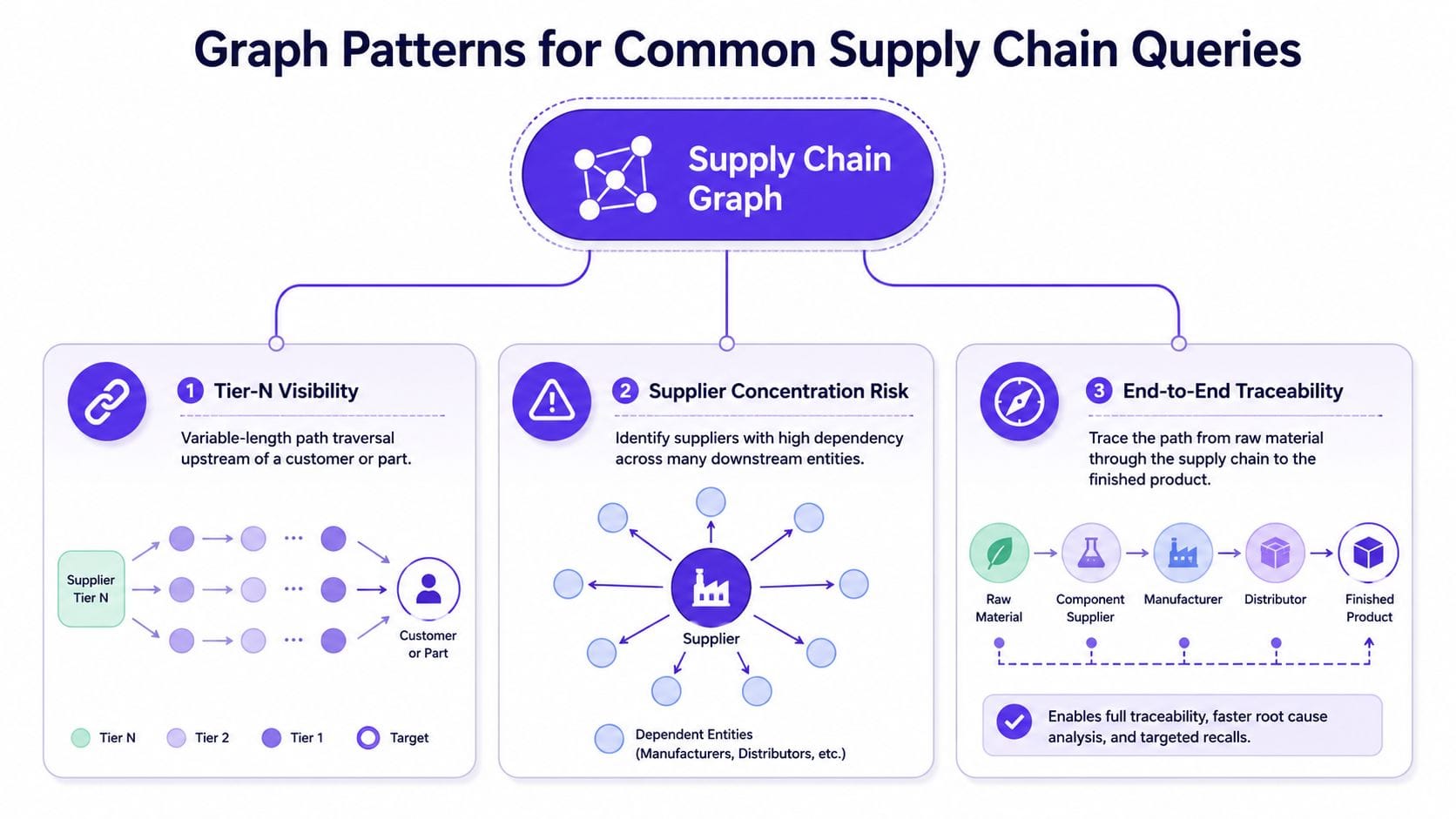
Supply chain teams ask a small number of questions over and over in different words. Underneath, they are three traversal shapes.
Here they are as queries.
1. Tier visibility
Walk upstream from a finished good through every level of the bill of materials and return the suppliers at each tier.
MATCH path = (:Product {sku: $sku})<-[:COMPONENT_OF*1..5]-(component:Part)
MATCH (s:Supplier)-[:SUPPLIES]->(component)
RETURN s.name            AS supplier,
       s.country         AS country,
       length(path)      AS tier,
       component.part_id AS part
ORDER BY tier, supplier;
The same question in SQL:
WITH RECURSIVE bom AS (
  SELECT child_part_id, parent_part_id, 1 AS tier
  FROM bill_of_materials
  WHERE parent_part_id = :sku
  UNION ALL
  SELECT b.child_part_id, b.parent_part_id, bom.tier + 1
  FROM bill_of_materials b
  JOIN bom ON b.parent_part_id = bom.child_part_id
  WHERE bom.tier < 5
)
SELECT s.name, s.country, bom.tier, bom.child_part_id
FROM bom
JOIN supplier_part sp ON sp.part_id     = bom.child_part_id
JOIN suppliers     s  ON s.supplier_id  = sp.supplier_id
ORDER BY bom.tier, s.name;
The SQL works. The point is not that it is impossible, it is what happens next. Going from five tiers to unbounded means restructuring the CTE and adding a visited-set cycle guard; in Cypher it is *1..5 to *. Adding “and which plants consume these parts, and which open orders those plants feed” is two more joins and a second recursion in SQL, and two more MATCH lines in Cypher. Depth and breadth are cheap to change in a traversal and expensive to change in a join tree, and supply chain questions change constantly.
2. Shipment lineage with provenance
Reconstruct a shipment leg by leg, and return the scan events that justify each hop.
MATCH (:Shipment {shipment_id: $shipmentId})-[h:HAS_LEG]->(leg:Leg)
MATCH (leg)-[:FROM]->(origin:Location)
MATCH (leg)-[:TO]->(dest:Location)
OPTIONAL MATCH (e:ScanEvent)-[:OBSERVED]->(leg)
RETURN h.seq          AS seq,
       leg.mode       AS mode,
       leg.carrier_scac AS carrier,
       origin.name    AS from_loc,
       dest.name      AS to_loc,
       collect({type: e.type, ts: e.ts, system: e.source_system}) AS evidence
ORDER BY seq;
The collect() is the important line. Every row comes back with the source events that produced it, including which system reported them. A leg with an empty evidence list is the gap: the missed handoff, returned as data rather than inferred by an analyst comparing three exports. This is also what makes the result safe to hand to an LLM, since the model has records to cite instead of a summary to embellish.
3. Supplier concentration risk
Fan out from every supplier to the open orders that depend on them, and rank by exposed value.
MATCH (s:Supplier)-[:SUPPLIES]->(:Part)-[:COMPONENT_OF*1..5]->(prod:Product)
      -[:FULFILLS]->(o:Order)
WHERE o.status = 'OPEN' AND o.due_ts <= $horizon_ts
WITH s,
     count(DISTINCT prod) AS products_at_risk,
     count(DISTINCT o)    AS open_orders,
     sum(o.value)         AS exposed_value
WHERE products_at_risk > 1
RETURN s.name    AS supplier,
       s.country AS country,
       products_at_risk,
       open_orders,
       exposed_value
ORDER BY exposed_value DESC
LIMIT 20;
This is a traversal with aggregation at the boundary rather than a table scan, and the shape matters: the expensive part is the variable-length BOM expansion, not the aggregation. That is why concentration scoring is usually the first query to fall over on a relational stack at real BOM depth, and why it is a good candidate for the first workload in a migration.
4. Disruption propagation
Given an incident, find everything downstream of it within four hops.
MATCH (:Incident {incident_id: $incidentId})-[:AFFECTS]->(root:Supplier)
MATCH path = (root)-[:SUPPLIES|COMPONENT_OF|CONSUMED_BY*1..4]->(downstream)
WHERE downstream:Product OR downstream:Plant
RETURN labels(downstream)[0]                     AS kind,
       coalesce(downstream.sku, downstream.name) AS entity,
       min(length(path))                         AS hops_from_incident,
       count(path)                               AS dependency_paths
ORDER BY hops_from_incident, dependency_paths DESC;
Two columns carry the analysis. hops_from_incident is how directly the exposure runs. dependency_paths is how many independent routes connect the two, which is the difference between an entity that has one fragile link to the incident and one that is entangled with it. A single-hop dependency with one path is a substitution problem. A three-hop dependency with forty paths is a redesign problem.
Note the :Supplier label on root. AFFECTS can also point at a :Location, and a location-rooted incident (a port closure, a flooded DC) propagates through the movement subgraph rather than the sourcing one, so it needs a different traversal starting at (:Location)<-[:TO]-(:Leg)<-[:HAS_LEG]-(:Shipment). Leaving root unlabelled would not error. It would quietly return nothing for exactly the incidents most likely to trigger the query.
SQL can express this with recursive CTEs. It gets brittle quickly, because the traversal has to stay explainable to the planner who is going to act on it, and a four-level CTE with mixed edge semantics stops being readable well before it stops being correct.
5. Hybrid retrieval: find the failure mode, then find the exposure
This is the query that justifies putting vectors and traversal in the same engine. A planner describes a failure in their own words. The system finds semantically similar past incidents, then walks the current network to see who is exposed to the same entities today.
CALL db.idx.vector.queryNodes('Incident', 'embedding', 10, vecf32($queryVector))
YIELD node AS similar, score
MATCH (similar)-[:AFFECTS]->(root:Supplier)
MATCH (root)-[:SUPPLIES|COMPONENT_OF*1..3]->(p:Product)-[:FULFILLS]->(o:Order)
WHERE o.status = 'OPEN'
RETURN similar.summary                     AS past_incident,
       score,
       root.name                           AS shared_supplier,
       collect(DISTINCT p.sku)[0..5]       AS sample_products,
       count(DISTINCT o)                   AS open_orders_exposed
ORDER BY score DESC;
$queryVector arrives from the driver as a plain float array; vecf32() casts it to the 32-bit float vector the index is built on. Some clients will do that coercion for you, so check your driver before assuming the cast is redundant. Passing an uncast array against a vecf32 index is the kind of mismatch that surfaces as an empty result set rather than an error.
One query, one engine, one identity space. The vector search finds the entry point when the language is messy. The traversal supplies the exact network context once the entry point is found.
Split these across a vector store and a warehouse and you are joining on supplier IDs across two systems at request time, hoping both were reconciled by the same ETL run. The failure is quiet: the vector store matches “Nordwerk Präzision GmbH” and the warehouse joins on SUP-4471, and nobody finds out they diverged until an incident makes the gap expensive.
Requirements that decide which database survives production
A demo looks convincing with a small dataset and one user. Production adds planners, agents, analysts, and integration jobs hitting the same store simultaneously, and the constraints show up in a specific order.
Latency is tiered, not a single number
Interactive agent tool calls need to return fast enough that a conversation feels live, which in practice means double-digit milliseconds per call, because an agent may issue five or six of them before it answers. Dashboards tolerate a second or two. Batch risk scoring can run for minutes. These are three different budgets, and a platform that forces all three through one path lets the slowest one set the pace.
Query 3 above is the one to benchmark, not a single-hop lookup. Vendor benchmarks are usually run on shapes that flatter the engine; the honest test is your own concentration query at your own BOM depth.
Multi-tenancy determines unit economics
Supply chain software is usually delivered to many customers or business units from one platform. Giving each one a dedicated database instance pushes cost, deployment complexity, and upgrade coordination up on a per-customer basis, which means every new logo is an infrastructure project. Native tenant isolation inside a single cluster keeps density high without giving up the boundary.
Write pressure is continuous
Shipment state never sits still. EDI feeds, partner APIs, IoT telemetry, and warehouse scans arrive constantly, and the database has to absorb them without starving reads. A batch-only design tests fine and fails during the incident it was bought for, because the graph is reasoning over yesterday’s network at the moment freshness matters most.
Provenance is a schema decision, not a feature
Every answer should trace back to the source event that produced it. This is not something a database gives you; it is something you model, as in the ScanEvent structure above. The database’s job is to make carrying that evidence cheap enough that nobody strips it out for performance.
Scale has two axes
Graph size and write volume fail independently. A network can reach millions of nodes and edges per tenant while the ingest path stays modest, or stay small while events stream in continuously. Load-test both, separately.
Vendor check: ask how the platform handles provenance, write bursts, and tenant isolation together. If you get three separate answers, the architecture is three separate systems.
The KPI layer sits on top of all of this. Order fill rate, perfect order rate, on-time delivery, inventory turnover, supplier lead time, and days of inventory on hand are the standard set, and they are simple to define and hard to keep aligned across ERP, WMS, transportation, and partner data. Aligning them is an entity resolution problem before it is a metrics problem, which is a useful thing to discover before rather than after you build the dashboard. Master data practice covers the discipline side of this well; supply chain master data guidance is a reasonable starting point.
Integration patterns for RAG, agents, and analytics
One database can feed three very different consumers, but only if identity and provenance live in one place. Split the network across a warehouse, a vector store, and a search index, and each consumer sees a slightly different version of the truth. That drift is where AI systems start hallucinating around the edges of a real logistics problem, not by inventing facts outright but by confidently joining two records that were never the same entity.
RAG needs entity-anchored context. Retrieval should return suppliers, shipments, incidents, and the edges between them, not a blob of adjacent text. Query 2 is a good template: the response carries the records and the evidence that produced them, so the model has something to cite. When retrieval is grounded in records, a wrong answer is auditable. When it is grounded in text chunks, it is not.
Agents need a schema-aware tool interface. Natural language to Cypher works well when the agent is constrained to a typed schema and returns typed results, because it can reason over the answer without guessing at column names. The database becomes a tool backend rather than a passive store. The same design shows up in graph-backed chatbots, where retrieval and generation stay tied to the underlying graph.
Analytics uses the same graph in a different mode. Concentration scoring, anomaly detection, and propagation analysis are the same traversals run in bulk rather than interactively. Routing and movement problems reduce to graph work too; see vehicle routing problems for a worked example of the same principle in a different shape.
The advantage of one backend is operational, not ideological. Permissions stay consistent, entity identity stays consistent, and provenance stays consistent, because there is one place for each to be defined.
Migration: from a warehouse, and from Neo4j
From a warehouse
Start with one hard question, not a platform rewrite. Supplier concentration and shipment lineage are the usual first choices, because business teams understand them immediately and they are the two that tables handle worst. Model only the nodes and edges that question needs, prove the workload, then expand.
Keep the system of record in place. The graph can run beside it as a derived layer for analytics and AI while the warehouse continues to own transactional truth. That lowers cutover risk to roughly zero and gives you a way to validate query coverage before anyone commits to scope.
Use change data capture rather than nightly rebuilds. A batch-refreshed graph looks fine in staging and is worthless during a live incident, which is the scenario that justified the project.
Budget real time for entity resolution. Duplicate supplier names, inconsistent location codes, and mismatched part identifiers do not degrade traversals gracefully. They silently split one entity into two, and every downstream count is wrong in a way nobody notices. Resolve identity before you load, not after. If you are coming from a purely relational mindset, relational database to graph database covers the modeling shift: relationship shape belongs in the data model rather than hidden behind foreign keys.
Migration heuristic: measure success by query coverage and response time on the target use case, not by how much raw data you loaded in week one.
From Neo4j
This migration is mostly mechanical, because both speak Cypher. Most read queries port unchanged. Budget your time for the four places where they diverge.
Inventory your APOC usage first. This is usually the largest single item. FalkorDB does not ship APOC, so every apoc.* call needs either a plain-Cypher equivalent or application-side logic. Export and import procedures are the most common dependency and the easiest to replace; graph-manipulation procedures take longer.
Inventory your GDS usage second. Graph Data Science algorithms do not port by name. FalkorDB provides its own procedures for the common graph algorithms, so check coverage for the specific ones you rely on. Pathfinding and centrality are well covered, and anything exotic should be verified against current docs before you commit to a date.
Check type usage. Temporal and spatial type support differs between the two. Queries built on rich date arithmetic or point geometry need review. Storing timestamps as epoch integers, as in the due_ts and ts properties above, sidesteps the issue entirely and is worth doing regardless.
Rethink the tenancy model. Neo4j’s database-per-tenant pattern maps onto FalkorDB’s multiple graphs in a single instance. This is usually the reason teams are migrating, so it is worth modeling deliberately rather than porting the old structure over.
For the cutover itself: export nodes and relationships to CSV, load with the bulk loader for the initial population, then run both systems in parallel with query-level output diffing on your top twenty queries until the diff is empty. Parallel running is what turns this from a migration into a switch.
How FalkorDB fits
A supply chain graph has to do two things at once: walk the network fast enough for interactive AI, and stay explainable enough for planners and auditors. Those pull in opposite directions, and FalkorDB is built around that tension.
Traversal performance. The engine represents adjacency as sparse matrices and executes traversals as linear algebra, which is what keeps multi-hop queries efficient when an agent issues several of them inside a single interaction.
The concentration query is the one worth quoting a number on, because it is the shape that breaks first. On internal benchmarks, Query 3 walking a five-tier BOM across a graph of 2.5 million nodes and 10 million edges returns at a p99 under 12ms. At that budget an agent can issue five or six traversals inside one interaction and still answer before the planner notices it is thinking. Run it on your own BOM depth before you believe anyone’s number, including ours.
Multi-tenant isolation. Multiple isolated graphs in one instance means tenant boundaries without per-tenant infrastructure. For a SaaS supply chain platform, this is the difference between onboarding a customer and provisioning a cluster.
Graph and vector in one engine. Query 5 is the demonstration. Traversal supplies exact network context, vector search recovers the right entry point when the user’s language is messy, and both run against the same identity space in a single query rather than a two-system join at request time.
The unglamorous layer. Cloud clustering across AWS, GCP, and Azure, TLS, VPC peering, rolling upgrades, and automated backups with a documented recovery point objective. None of it is interesting until the first production incident, at which point it is the only thing that matters. The question to ask any vendor, including this one, is not whether backups exist but what the RPO actually is and who has tested a restore recently.
For teams comparing options, the evaluation reduces to three questions. Can the database answer multi-hop lineage and propagation queries at interactive latency on your real BOM depth? Can it ground AI retrieval in explicit entities with provenance attached? Can it hold tenant boundaries under continuous write load? A no on any one of them rules it out for this workload.
The queries in this guide run as written. If you want to try them against your own network, start a free instance and load a slice: one product family, its BOM, and ninety days of shipment events is enough to see whether the traversals hold up at your depth.
