


Orders are piling up, dispatch is juggling driver calls, and the route plan that looked fine at 6 a.m. is already wrong by 8. One customer needs a tighter delivery window. Another added a pickup. A driver is close to capacity. Traffic changed the practical route even if the map still shows the shortest path.
That’s the moment when vehicle routing problems stop being academic and start becoming operational. Teams usually begin with spreadsheets, fixed territories, or a basic shortest-path tool. Those approaches work until the business adds more stops, more constraints, and more real-time change than a manual planner can absorb.
The hard part isn’t drawing lines on a map. It’s deciding which vehicle should serve which customer, in what sequence, under which constraints, and with what trade-off between cost, service, and resilience. Classical operations research gives the modeling discipline for that. Modern graph systems and AI make it easier to implement, update, and operationalize those models in production.
Table of Contents
- What Are Vehicle Routing Problems
- Understanding Common VRP Variants
- How to Model VRPs and Define Objectives
- Navigating Solution Methods from Exact to AI
- Implementing VRP Solutions with Graph Databases
- Advanced Patterns and Performance in FalkorDB
- The Future of Routing is Autonomous and Graph-Powered
What Are Vehicle Routing Problems
A vehicle routing problem, or VRP, is the problem of finding the best set of routes for a fleet of vehicles to serve a set of customers from one or more depots. “Best” depends on the operation. It might mean lower distance, better on-time performance, fewer vehicles, less overtime, or a balance of all four.
The reason VRP matters so much is simple. Real fleets don’t fail because they can’t find roads. They fail because operating constraints collide. A truck can reach a customer, but not within the promised time. A driver can take one more stop, but not one more pallet. A pickup is physically close, but adding it breaks the rest of the day.
VRP entered operations research formally in 1959, when George Dantzig and John Ramser introduced it in The Truck Dispatching Problem, applying optimization to petrol deliveries for a gasoline distribution company (vehicle routing problem history). That paper is still the right mental starting point because the core question hasn’t changed: given customers, vehicles, and constraints, what set of routes should the fleet run?
Three ingredients appear in almost every practical model:
- Vehicles with limits such as capacity, shift duration, equipment, or service region
- Customers or stops with demands, service times, and sometimes time commitments
- Depots or start points where routes begin, and sometimes where they must end
Practical rule: If dispatchers are repeatedly overriding the “optimized” plan, the problem usually isn’t bad driver behavior. It’s an incomplete model.
For teams working through the operational side of this, a grounded overview of route planning for hauliers is useful because it frames routing as a planning system, not just a map feature.
Understanding Common VRP Variants
Most failed routing projects don’t fail because the solver is weak. They fail because the team modeled the wrong variant.
A grocery van, a field service fleet, and a medical sample pickup network all look like “delivery routes” at a distance. In practice, they are different optimization problems. The route pattern changes because the constraint set changes.
The base VRP and why variants matter
The base VRP asks for routes that visit all customers while minimizing a routing objective under fleet rules. That’s fine for a conceptual start. It’s rarely enough for production.
The first modeling question I’d ask any team is this: what causes a human planner to reject an otherwise short route? The answer usually reveals the variant. If the answer is “the van can’t hold that much,” you are in capacity territory. If it’s “the customer only accepts between specific hours,” you’re in time-window territory. If it’s “we deliver first, then collect returns,” you’re dealing with pickup and backhaul structure.
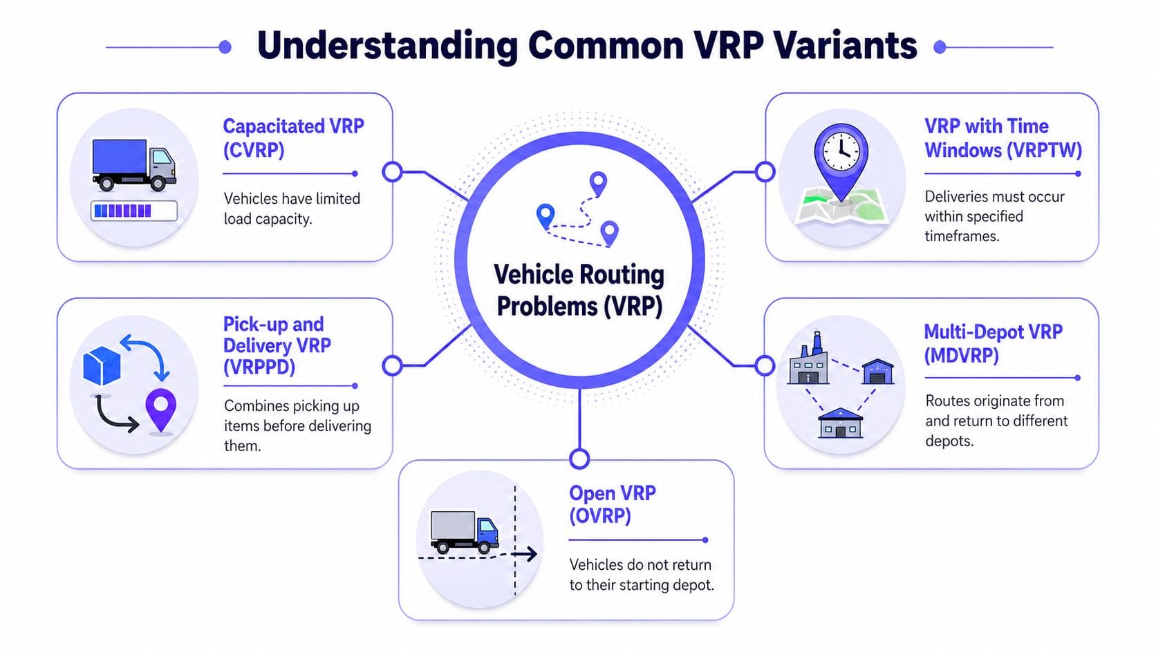
Capacitated VRP
In Capacitated VRP, each vehicle has a finite carrying limit and each customer consumes some of that capacity. This is the workhorse model for parcel, grocery, beverage, retail replenishment, and many distribution operations.
The key point isn’t just that vehicles have limits. It’s that capacity changes route composition. A route that is geographically compact may still be infeasible because the early stops fill the truck too quickly. Good models account for that before the route is ever shown to a dispatcher.
Common examples include:
- Parcel fleets: Van cube and weight matter as much as street distance.
- Retail distribution: Heavy and bulky drops can distort what looks like the best cluster on the map.
- Food service: Temperature zones or compartment rules can act like extra capacity dimensions.
A common mistake is to treat capacity as a post-check. That leads to frequent rework because the solver first finds an attractive path and only later discovers the truck can’t execute it.
VRP with Time Windows
In VRP with Time Windows, each stop must be served within an allowed interval. That interval might be strict, like a store receiving slot, or softer, like a promised arrival band.
This variant forces the planner to think in time, not just distance. A nearby customer can be expensive if serving them early creates idle time, or if serving them late breaks the route. Time windows also interact with service duration. A stop with unloading, signature, inspection, or handoff time can consume far more route capacity than its driving time suggests.
Short routes often lose to well-timed routes. Dispatchers learn this early. Solver configurations need to learn it too.
Practical cases include B2B distribution, home services, technician scheduling, and healthcare visits. In all of them, the route sequence determines whether the day is feasible.
VRP with Backhauls and pickup flows
Backhaul problems are where many implementations get sloppy. Teams say “pickup and delivery” as if that were one generic feature. It isn’t. The order structure matters.
In VRP with Backhauls, the fleet typically starts from a single depot, performs linehaul deliveries, and then handles pickup activity. The initialization step matters more than many guides admit. A documented approach uses seed radials uniformly located around the distribution center using ring-radial distance metrics to define initial route clusters before optimization heuristics are applied (vehicle routing problem with backhauls).
That matters operationally because bad clustering at the start produces bad route shapes later. If you mix delivery and pickup geography too early, routes become hard to balance and harder to execute.
Here’s where backhaul logic helps:
- Returns collection: Deliver outbound goods first, then collect empties or returns on the return leg.
- Medical sample transport: Scheduled deliveries may need to precede pickup activity to protect handling sequences.
- Retail reverse logistics: Store replenishment and unsold-goods collection often share the same fleet but not the same route phase.
Comparison of common VRP variants
| Variant | Primary Constraint | Example Use Case |
|---|---|---|
| CVRP | Vehicle load capacity | Grocery or parcel delivery vans |
| VRPTW | Customer service time windows | B2B delivery appointments |
| VRPB | Delivery and pickup sequencing from a depot | Returns collection after store deliveries |
How to Model VRPs and Define Objectives
A routing model becomes useful when it reflects an operating decision that someone finds valuable. If the business says “cut route cost,” but dispatch overrides the plan to protect service promises, then cost wasn’t the primary objective. The model and the operation are misaligned.
Start with the operating decision
Every VRP model has three moving parts:
- Decision variables that represent choices, usually which vehicle travels between which stops and in what order.
- Constraints that encode what’s allowed.
- An objective function that ranks feasible plans.
In plain terms, the objective is the answer to “what should the solver optimize first?” Minimize total distance is common, but it’s only one option. In formal terms, a standard objective is to minimize total travel cost, for example $min sum c_{ij} x_{ij}$, subject to capacity, visit, and time-feasibility constraints. Teams also optimize for service reliability, route balance, vehicle count, or a weighted blend.
A key pitfall is pretending uncertainty doesn’t exist. In stochastic vehicle routing problems, where demand or travel times are uncertain, optimal solutions often require a 15 to 25% increase in total fleet distance compared with deterministic counterparts to maintain a 95% service-level probability (stochastic VRP benchmark data). That’s exactly why a route that looks efficient on yesterday’s averages can fail in today’s operation.
Turn business rules into solver constraints
A practical model usually includes rules like these:
- Capacity constraints: A vehicle can’t exceed its load limit.
- Visit constraints: Every customer must be served, unless the model explicitly allows optional drops.
- Time feasibility: Travel and service must fit within customer and driver windows.
- Start and end rules: Vehicles may return to depot, finish elsewhere, or hand off work.
A useful way to pressure-test the model is to write constraints in operational language before writing code. “This truck can’t run beyond its shift.” “This stop can only be served in the afternoon.” “This pickup must happen after a delivery phase.” If the planner can’t state the rule clearly, the solver won’t rescue the design.
For teams dealing with disruptions around major logistics bottlenecks, the 2026 haulier survival guide is a good reminder that the routing objective often has to absorb external volatility, not just distance minimization.
If planners add manual buffer everywhere, the model is missing uncertainty. If the solver adds buffer everywhere, the objective is too defensive.
Navigating Solution Methods from Exact to AI
A dispatcher has 12 vehicles on the road, a few hundred stops queued, and new exceptions arriving every few minutes. At 2 a.m., an exact model that proves optimality is attractive. At 9:15 a.m., after two drivers call in sick and a customer shifts a delivery window, the better question is different: which method can produce a feasible, high-quality revision before the operation slips?
Why VRP gets hard fast
Vehicle routing is hard for the same reason the Traveling Salesman Problem is hard, then harder again once you add multiple vehicles, capacities, time windows, depot rules, and service constraints. The underlying complexity class is well established in the routing literature. Toth and Vigo’s Vehicle Routing: Problems, Methods, and Applications treats the capacitated VRP as NP-hard and discusses its close relationship to TSP-style combinatorial search (SIAM overview of VRP methods and complexity).
That matters operationally. Each added business rule cuts down the set of feasible routes, but it also makes the search space harder to explore efficiently. A planner sees “add driver breaks” as one more requirement. A solver sees a much tighter feasibility region and many more ways to get stuck.
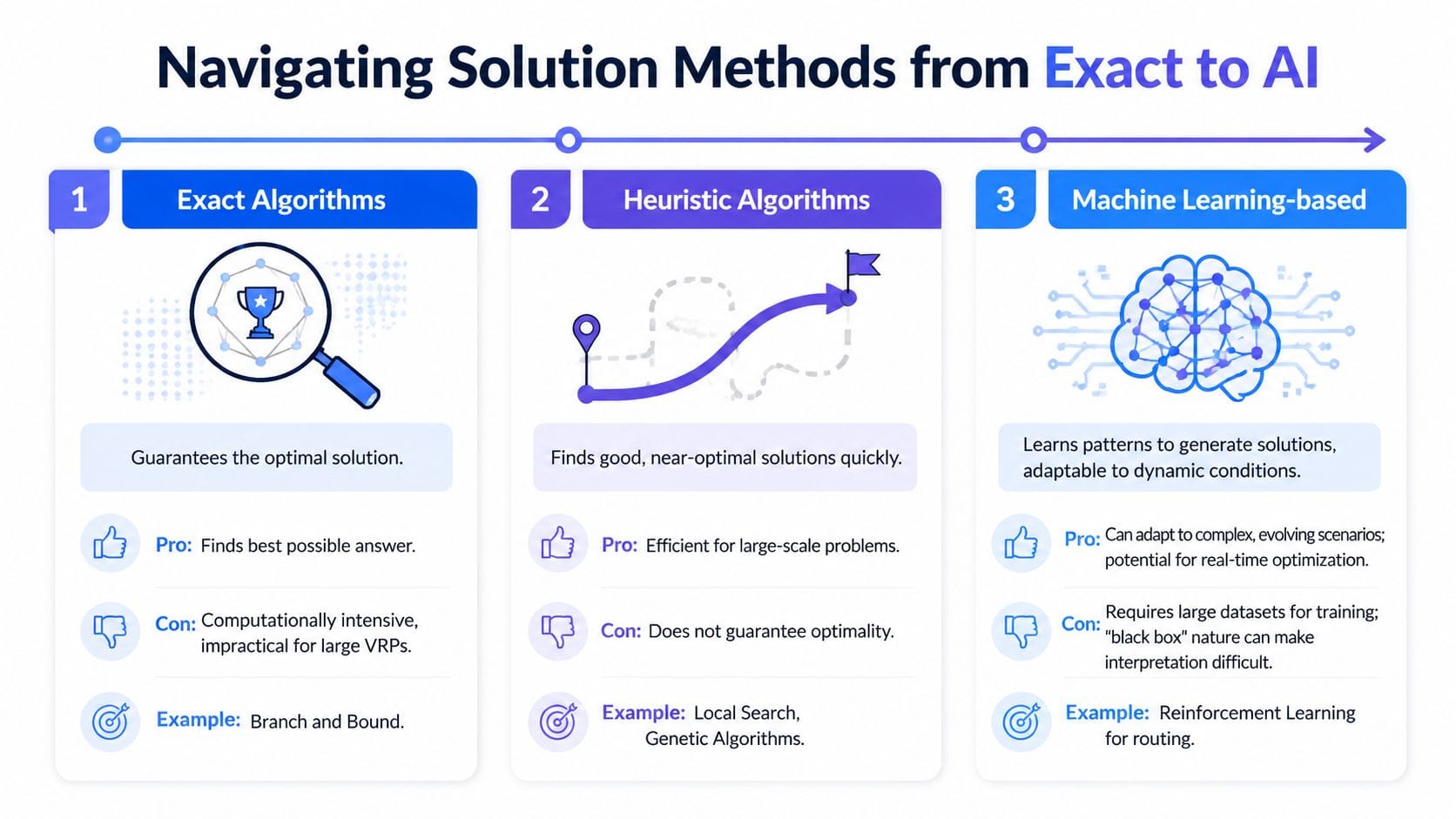
Exact methods
Exact methods are still the right tool in some cases. Mixed-integer programming, branch-and-cut, branch-and-price, and decomposition methods are built to prove optimality or prove that no feasible solution exists under the current model.
Use them when the answer needs legal, financial, or policy weight behind it. Network design studies, master route planning, contract evaluation, and benchmark generation are all good candidates. They are also useful during model development because small exact solves expose bad constraints quickly. If a 25-stop test case fails for reasons nobody can explain, the formulation usually needs work before the algorithm does.
The trade-off is runtime. Exact methods get expensive fast as the instance grows or as the input changes mid-execution. In production dispatch, a mathematically perfect answer that arrives after the cut-off is worse than a slightly weaker answer that keeps trucks moving.
Heuristics and metaheuristics
Heuristics carry most real routing systems. They give up proof of optimality in exchange for speed, controllability, and repeatability.
Classical methods still matter here. Clarke-Wright savings, sweep-based construction, insertion heuristics, and route-first cluster-second ideas remain useful because they create decent initial plans with very little compute. That initial plan is rarely the final answer. It is the starting point for local search moves such as 2-opt, relocate, exchange, cross, or more problem-specific repairs for time windows and load violations.
Metaheuristics widen that search. Tabu search, simulated annealing, large neighborhood search, and genetic algorithms help the solver escape weak local minima and keep improving after simple local search stalls. The practical issue is tuning. Penalty weights, neighborhood definitions, acceptance criteria, and restart logic all affect whether the method behaves well on your data or burns time exploring moves that planners would reject immediately.
A pattern I trust in production is simple: build fast, improve selectively, repair aggressively, and stop on time. If the operation replans every 15 minutes, the search strategy has to respect that cadence.
For large territories, clustering often helps before route construction starts. Geographic clustering is not the routing solution by itself, but it can reduce search cost and create cleaner subproblems. This comparison of graph clustering algorithms for connected optimization workloads is useful if the implementation sits on a graph stack rather than a flat distance matrix.
Learning-based methods
Machine learning changes where computation goes. It does not remove the need for a formal routing model.
The strongest systems I have seen use OR to enforce feasibility and use learning where estimation or search guidance is the core challenge. That can mean predicting travel times from live conditions, ranking promising insertion moves, selecting destroy-and-repair neighborhoods, or deciding when to reoptimize instead of rebuilding the whole plan. In other words, AI is often best as a policy layer around the solver, not as a replacement for constraints.
This is the gap many academic writeups leave open. They explain the algorithm but not the implementation pattern. In a modern stack built on a property graph, the graph stores the current operational state, the solver enforces route feasibility, and an AI layer can reason over changing context, exceptions, and historical outcomes. That architecture fits tools like FalkorDB and GraphRAG well because both depend on connected state rather than isolated records.
How to choose the right family
Use exact methods for bounded problems where proof matters more than turnaround time.
Use heuristics and metaheuristics for day-to-day planning where the business needs good routes on a deadline.
Use hybrid AI methods when the network changes continuously and the main value is faster adaptation, better estimates, or smarter search control.
The common failure mode is choosing based on trend instead of workload. Teams adopt machine learning before they have a stable objective, clean event data, or a reliable way to score route quality. In that situation, a disciplined heuristic pipeline usually performs better and is easier to trust.
Good routing systems are built in layers. Classical OR defines the feasible region. Heuristics search it efficiently. Graph infrastructure keeps the state connected. AI helps the system react when conditions are no longer static.
Implementing VRP Solutions with Graph Databases
A lot of routing implementations break because the data model fights the problem. Teams store locations in one table, road costs in another, vehicle attributes in a third, live events in a queue, and route state somewhere else. Then they ask the application layer to reconstruct connectivity and context each time the plan changes.
A property graph is often a better fit because routing is natively about entities and relationships.
Why a property graph fits routing naturally
In a graph model:
- Depots, customers, and vehicles become nodes.
- Road connections, assignments, and route legs become edges.
- Distance, travel time, demand, capacity, and status become properties.
That structure maps cleanly to how dispatchers think. “Vehicle A is assigned to Route B.” “Customer C is near Depot D.” “This edge is blocked.” “This stop has a time window.” You’re working with connected facts instead of reconstructing joins every time the route changes.
If you want a broader primer on why this model works well beyond routing, this explanation of a graph database explained is worth reading.
A practical graph model for VRP
A simple production-friendly schema might look like this:
- (:Depot) with properties like
id,name, and operating hours - (:Customer) with
id,demand,service_time, and time-window fields - (:Vehicle) with
id,capacity, shift metadata, and equipment tags - [:ROAD] edges with
distance,travel_time, and maybe a current status flag - [:ASSIGNED_TO] edges linking vehicles to depots or route plans
- [:SERVES] edges recording actual or proposed visit order
That gives you two important capabilities. First, you can prepare solver inputs from graph traversals and property filters. Second, you can write optimized routes back into the same graph and query them operationally.
A simple Cypher example
Below is a compact example of how a VRP graph can be represented in Cypher:
CREATE (d:Depot {id: 'D1', name: 'Main Depot'})
CREATE (c1:Customer {id: 'C1', demand: 12, service_time: 15})
CREATE (c2:Customer {id: 'C2', demand: 8, service_time: 10})
CREATE (v:Vehicle {id: 'V1', capacity: 20})

CREATE (d)-[:ROAD {distance: 6, travel_time: 12}]->(c1)
CREATE (c1)-[:ROAD {distance: 4, travel_time: 9}]->(c2)
CREATE (c2)-[:ROAD {distance: 7, travel_time: 14}]->(d)

CREATE (v)-[:ASSIGNED_TO]->(d);
And a basic query to find reachable customers from a depot might be:
MATCH (d:Depot {id: 'D1'})-[:ROAD]->(c:Customer)
RETURN c.id, c.demand, c.service_time;
To show why graphs are especially useful for active route plans, you can also represent stop order directly in the graph:
CREATE (v)-[:NEXT_STOP {route_id: 'R1', seq: 1}]->(c1)
CREATE (c1)-[:NEXT_STOP {route_id: 'R1', seq: 2}]->(c2)
CREATE (c2)-[:NEXT_STOP {route_id: 'R1', seq: 3}]->(d)
Then traversal becomes simple. You can inspect the current sequence for a vehicle, validate the next handoff, or rewrite only the affected leg when dispatch changes the plan:
MATCH (v:Vehicle {id: 'V1'})-[:NEXT_STOP*]->(stop)
RETURN stop.id;
That isn’t a solver. It is the right substrate for one. The graph stores the operational world in a way that makes route generation, re-evaluation, and explanation easier.
Advanced Patterns and Performance in FalkorDB
Once the basics are working, the hard problems return. Orders change after dispatch. Travel conditions shift. Drivers leave comments about difficult sites. A route that is mathematically feasible becomes operationally ugly because paths intersect, vehicles conflict, or a stop should be avoided for reasons hidden in text rather than structured fields.
That’s where graph-native patterns become much more interesting than a plain “run solver, export route” loop.
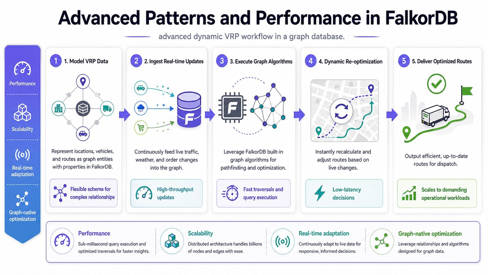
Use the graph as the operational control plane
A strong production pattern is to separate responsibilities cleanly:
- The graph stores the live state of depots, customers, vehicles, roads, assignments, and route history.
- The solver consumes a current subgraph that reflects what’s feasible right now.
- The application writes route decisions back as ordered relationships and status updates.
This works well because the graph becomes the shared operational context. You don’t have to rebuild state from scattered stores before every re-optimization. You query the current network, solve against it, and persist the result where downstream services can inspect it.
When teams care about latency under changing workloads, benchmark-oriented reading like graph database performance benchmarks comparing FalkorDB and Neo4j helps frame why engine behavior matters for live routing systems.
GraphRAG for context-aware routing
Classical VRP models mostly optimize over structured data. Modern operations rarely live on structured data alone.
Driver notes, customer complaints, site access instructions, incident descriptions, and delivery exceptions often sit in tickets, logs, or message streams. Those records are full of routing signal. “Loading dock closed after noon.” “Tight turn for large vehicle.” “Security check causes delay.” “Repeated failed access.”
A GraphRAG pattern can connect those unstructured signals to graph entities such as customer nodes, site entrances, vehicles, or route segments. Then the routing service can retrieve both topology and context before suggesting a route adjustment.
That opens up a more useful decision style:
- Structured filter: exclude infeasible vehicles or blocked edges
- Graph retrieval: pull nearby alternatives, predecessor stops, or related route segments
- Context retrieval: bring in notes, incidents, and semantic similarity from text
- Decision layer: recommend a route change with an explanation dispatch can inspect
This isn’t about handing the wheel to an LLM. It’s about using AI retrieval to surface operational context that a standard objective function misses.
A route can be shortest and still be wrong. Context is often the missing variable.
Handling route crossings and live conflicts
Many tutorials stop after generating a sequence of stops. Real systems need to care about route geometry too.
A recurring issue in dynamic routing is crossing lines. A route may contain intersecting legs that are visually messy, operationally confusing, or inefficient. In static planning, teams often clean that up with 2-opt. In live systems, that can be too expensive to keep applying as concurrency rises. A documented gap in common guidance is the need for geometric intersection detection in real time, especially for agentic systems managing multiple vehicles (eliminating crossing lines in routing problems).
In practice, that changes the implementation:
- Detect intersections early: Treat crossing checks as part of runtime validation, not just post-processing.
- Repair locally when possible: Small swaps or route segment adjustments are often cheaper than full re-optimization.
- Account for fleet interaction: One vehicle’s tidy route can create spatial conflict for another if the system optimizes in isolation.
For multi-vehicle operations, I’d treat crossing detection as a first-class production concern, especially when routes update continuously.
Performance patterns that matter in production
A few design choices consistently separate toy routing systems from production ones:
- Subgraph extraction over whole-network solving: Solve on the relevant operational slice, not the entire graph.
- Incremental writes: Update only the affected route legs and assignment state when a change lands.
- Separation of feasibility and ranking: First remove impossible choices, then score the remaining candidates.
- Explainable route state: Persist why an edge or stop was chosen, skipped, delayed, or penalized.
The graph database is especially useful here because the same representation supports planning, execution, audit, and retrieval. You’re not just computing a route. You’re maintaining a connected decision record that other systems can query.
The Future of Routing is Autonomous and Graph-Powered
A dispatcher starts the day with a valid plan, then traffic shifts, a driver calls out, a customer changes a delivery window, and the original route is already stale. That is the operating reality modern routing systems have to handle. The future of VRP is not a single better solver. It is a routing stack that can keep recomputing decisions against live operational state without losing control of cost, feasibility, or explainability.
The core math still matters. Classical OR gives routing systems their discipline: explicit constraints, clear objectives, and repeatable behavior under pressure. Heuristics remain part of the job because production teams need answers on operational timescales, not just theoretically stronger solutions. AI adds another layer by helping systems interpret messy context, retrieve relevant operational knowledge, and propose adjustments when the problem changes faster than a batch optimizer can keep up.
That shift is why graph-based implementation matters so much in practice.
A property graph can hold the road network, vehicles, stops, time windows, skills, exceptions, and route history in one connected model. That closes a gap that academic VRP material often leaves open. The solver logic is only part of the system. Teams also need a representation that supports continuous updates, graph traversal, retrieval for downstream agents, and auditability when someone asks why a route was changed at 10:17 a.m. rather than 10:05.
That is where the OR-to-production handoff usually fails. Research papers explain formulation quality. Engineering teams still have to build the state model, connect it to live events, and expose it to AI systems that can reason over changing graph context. Combining property graphs with GraphRAG patterns gives developers a practical path from VRP theory to autonomous decision support. The graph stores the operational truth. Retrieval and agents use that graph state to explain, revise, and coordinate actions without treating routing as an isolated optimization run.
The next generation of logistics systems will compute routes, monitor execution, revise assignments, and justify the trade-offs behind those decisions as conditions change. For teams building these next-generation systems, the underlying graph technology is the critical foundation.
When moving from theory to live execution, having a database engineered for fast traversal and contextual retrieval is essential. Platforms like FalkorDB, Inc. provide the graph foundation needed for modern GraphRAG and agentic routing workflows.
Written with Outrank
